Optimize Scope 2 Emissions
This tutorial will walkthrough how to optimize Scope 2 emissions for a simple battery model in either CVXPY or Pyomo by going through the following steps:
Load a Scope 2 emissions spreadsheet
Configure an optimization model of the electricity consumer with system constraints
Consider using flexibility metrics to encode system constraints (Flexibility Metrics as Constraints)!
The models are presented step-by-step to demonstrate the model building process, but the complete models are available in the examples folder:
Create an objective function of Scope 2 emissions using the emissions factors
Minimize the Scope 2 emissions of this consumer given the system constraints and base load consumption
Display the results to validate that the optimization is correct
CVXPY
Import dependencies
import datetime
import cvxpy as cp
import pandas as pd
import matplotlib.pyplot as plt
from electric_emission_cost.units import u
from electric_emission_cost import emissions
Load a Scope 2 emissions spreadsheet
path_to_emissions_sheet = "electric_emission_cost/data/emissions.csv"
emission_df = pd.read_csv(path_to_emissions_sheet, sep=",")

# get the charge dictionary
carbon_intensity = emissions.get_carbon_intensity(
    datetime.datetime(2023, 4, 9), datetime.datetime(2023, 4, 11), emission_df, resolution="1m"
)
We are going to evaluate the electricity consumption from only April 9th to April 10th since that is where our synthetic data comes from (https://github.com/we3lab/electric-emission-cost/blob/main/electric_emission_cost/data/consumption.csv). You will also see that it is in 1-minute intervals, hence resolution=”1m”.
Configure an optimization model of the electricity consumer with system constraints
# load historical consumption data
load_df = pd.read_csv("electric_emission_cost/data/consumption.csv", parse_dates=["Datetime"])

# set battery parameters
# create variables for battery total energy, max charge and discharge power, and SOC limits
total_capacity = 10 # kWh
min_soc = 0
max_soc = 1
init_soc = 0.5
fin_soc = 0.5
max_discharge = 5 # kW
max_charge = 5 # kW
T = len(load_df["Datetime"])
delta_t = ((load_df.iloc[-1]["Datetime"] - load_df.iloc[0]["Datetime"]) / T) / datetime.timedelta(hours=1)

# initialize variables
battery_output_kW = cp.Variable(T)
battery_soc = cp.Variable(T+1)
grid_demand_kW = cp.Variable(T)

# set constraints
constraints = [
    battery_output_kW >= -max_discharge,
    battery_output_kW <= max_charge,
    battery_soc >= min_soc,
    battery_soc <= max_soc,
    battery_soc[0] == init_soc,
    battery_soc[T] == fin_soc,
    grid_demand_kW >= 0
]
for t in range(T):
    constraints += [
        battery_soc[t+1] == battery_soc[t] + (battery_output_kW[t] * delta_t) / total_capacity,
        grid_demand_kW[t] == load_df.iloc[t]["Load [kW]"] + battery_output_kW[t]
    ]
This is a standard battery model with energy (i.e., total charge) and power (i.e., discharge/charge rate) constraints. The round-trip efficiency is 1.0 since there is no penalty applied when discharging the battery, but that’s fine for these demonstration purposes.
Create an objective function of Scope 2 emissions using the emissions factors
# NOTE: second entry of the tuple can be ignored since it's for Pyomo
obj, _ = emissions.calculate_grid_emissions(
    carbon_intensity,
    grid_demand_kW,
    resolution="1m",
    consumption_units=u.kW
)
There is also an optional emissions_units argument that we do not use in the above example. That is because get_carbon_intensity returns a pint.Quantity from which we can automatically parse the emissions units.
Minimize the Scope 2 emissions of this consumer given the system constraints and base load consumption
# solve the CVX problem (objective variable should be named obj)
prob = cp.Problem(cp.Minimize(obj), constraints)
prob.solve()
Display the results to validate that the optimization is correct
We will compare baseline to optimized emissions. Unlike Optimize Electricity Costs, there are no convex relaxations during problem formulation, so the objective function can be used directly to quantify emissions.
# NOTE: second entry of the tuple can be ignored since it's for Pyomo
baseline_emissions, _ = emissions.calculate_grid_emissions(
    carbon_intensity,
    load_df["Load [kW]"].values,
    resolution="1m",
    consumption_units=u.kW
)
# NOTE: second entry of the tuple can be ignored since it's for Pyomo
optimized_emissions = obj.value
If we print our results, we confirm that the optimal electricity profile has emissions of 9.74 kg CO:sub:2-eq, 0.95 kg CO:sub:2-eq less than the baseline emissions of 10.69 kg CO:sub:2-eq.
>>>print(f"Baseline Scope 2 Emissions: {baseline_emissions:.2f} kg CO_2-eq")
Baseline Scope 2 Emissions: 10.69 kilogram kg CO_2-eq
>>>print(f"Optimized Scope 2 Emissions: {optimized_emissions:.2f} kg CO_2-eq")
Optimized Scope 2 Emissions: 9.74 kilogram kg CO_2-eq
Below are a few simple plots to validate our results. First, we visualize the emissions factors:
fig, ax = plt.subplots()

# plot the emissions factors
ax.plot(load_df["Datetime"], carbon_intensity.to(u.kg / u.MWh))
ax.set(
    xlabel="DateTime",
    ylabel="Carbon Intensity (kg CO$_2$ / MWh)",
    xlim=(datetime.datetime(2023, 4, 9),
    datetime.datetime(2023, 4, 11)),
    ylim=[0,500]
)

fig.align_ylabels()
fig.tight_layout()
fig.suptitle("Scope 2 Emissions Factors",y=1.02, fontsize=16)
plt.show()
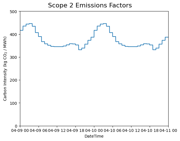
Average Scope 2 emissions factors for our modeling period (April 9-10, 2023).
Next, we plot the baseline and optimal electricity consumption profiles. This helps us to visualize how the model responds to the cost incentives of the tariff.
# plot the model outputs
fig, ax = plt.subplots()
ax.step(load_df["Datetime"], grid_demand_kW.value, color="C0", lw=2, label="Net Load")
ax.step(load_df["Datetime"], load_df["Load [kW]"].values, color="k", lw=1, ls='--', label="Baseload")
ax.set(xlabel="DateTime", ylabel="Power (kW)", xlim=(datetime.datetime(2023, 4, 9), datetime.datetime(2023, 4, 11)))
plt.xticks(rotation=45)
fig.tight_layout()
plt.legend()
plt.show()

Output of our electricity bill optimization using the virtual battery model. The dotted line is baseline electricity purchases, and the blue line is the optimized profile. Note how the optimized electricity profile shaves peaks to readuce time-of-use (TOU) charges
Finally, let’s plot the battery state of charge (SOC) to confirm that the constraints were respected:
# plot the battery charge
fig, ax = plt.subplots()
ax.step(load_df["Datetime"], battery_soc.value[1:], color="C1", lw=2, label="Battery SOC")
ax.set(
    xlabel="Time",
    ylabel="Battery SOC",
    ylim=[0,1],
    xlim=(datetime.datetime(2023, 4, 9), datetime.datetime(2023, 4, 11))
)
plt.xticks(rotation=45)
fig.tight_layout()
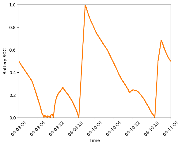
Battery state of charge (SOC) as a percentage during our modeling period (April 9-10, 2023).
Pyomo
Import dependencies
import datetime
import numpy as np
import pandas as pd
import matplotlib.pyplot as plt
from electric_emission_cost.units import u
from electric_emission_cost import emissions
from examples.pyomo_battery_model import BatteryPyomo
Load a Scope 2 emissions spreadsheet
path_to_emissions_sheet = "electric_emission_cost/data/emissions.csv"
emission_df = pd.read_csv(path_to_emissions_sheet, sep=",")

# get the charge dictionary
carbon_intensity = emissions.get_carbon_intensity(
    datetime.datetime(2022, 7, 1), datetime.datetime(2022, 8, 1), emission_df, resolution="15m"
)
We are going to evaluate the electricity consumption for the entire month of July 2022. Below we will create synthetic baseload data for this month with 15-minute resolution, so resolution=”15m”.
Configure an optimization model of the electricity consumer with system constraints
We rely on the virtual battery model in pyomo_battery_model.py. We’re going to stick to the electricity cost calculation details, but we encourage you to go check out the code to better understand the model.
# Define the parameters for the battery model
battery_params = {
    "start_date": "2022-07-01 00:00:00",
    "end_date": "2022-08-01 00:00:00",
    "timestep": 0.25,   # 15 minutes defined in hours
    "rte": 0.86,
    "energycapacity": 100,
    "powercapacity": 50,
    "soc_min": 0.05,
    "soc_max": 0.95,
    "soc_init": 0.5,
}

# Create a sample baseload profile based on a sine wave
baseload = np.sin(np.linspace(0, 4 * np.pi, 96))*100 + 1000 + np.random.normal(0, 10, 96)

# Create an instance of the BatteryOpt class
battery = BatteryPyomo(battery_params, baseload, baseload_repeat=True)

# create the model on the instance battery
battery.create_model()
The above code initializes the battery model with flexibility metrics like round-trip efficiency (RTE), power capacity, and energy capacity.
Create an objective function of Scope 2 emissions using the emissions factors
# compute Scope 2 emissions using Pyomo variable
battery.model.emissions, battery.model = emissions.calculate_grid_emissions(
    carbon_intensity,
    battery.model.net_facility_load,
    resolution="15m",
    consumption_units=u.kW,
    model=battery.model
)
# create an attribute objective based on the emissions
battery.model.objective = pyo.Objective(
    expr=battery.model.emissions,
    sense=pyo.minimize,
)
Minimize the Scope 2 emissions of this consumer given the system constraints and base load consumption
# use the glpk solver to solve the model - (any pyomo-supported LP solver will work here)
solver = pyo.SolverFactory("glpk")
results = solver.solve(battery.model, tee=False) # turn tee=True to see solver output
Display the results to validate that the optimization is correct
We will compare baseline to optimized emissions. Unlike Optimize Electricity Costs, there are no convex relaxations during problem formulation, so the objective function can be used directly to quantify emissions.
# retrieve outputs from Pyomo model
net_load = np.array([battery.model.net_facility_load[t].value for t in battery.model.t])
baseload = np.array([battery.model.baseload[t] for t in battery.model.t])

# NOTE: second entry of the tuple can be ignored since it's for Pyomo
baseline_emissions, _ = emissions.calculate_grid_emissions(
    carbon_intensity,
    baseload,
    resolution="15m",
    consumption_units=u.kW
)
# NOTE: second entry of the tuple can be ignored since it's for Pyomo
optimized_emissions = pyo.value(battery.model.objective)
If we print our results, we confirm that the optimal electricity profile has emissions of 9.74 kg CO:sub:2-eq, 0.95 kg CO:sub:2-eq less than the baseline emissions of 10.69 kg CO:sub:2-eq.
>>>print(f"Baseline Scope 2 Emissions: {baseline_emissions:.2f} kg CO_2-eq")
Baseline Scope 2 Emissions: 276673.42 kilogram kg CO_2-eq
>>>print(f"Optimized Scope 2 Emissions: {optimized_emissions:.2f} kg CO_2-eq")
Optimized Scope 2 Emissions: 276416.54 kilogram kg CO_2-eq
Below are a few simple plots to validate our results. First, we visualize the emissions factors:
fig, ax = plt.subplots()

# plot the emissions factors
ax.plot(battery.t, carbon_intensity.to(u.kg / u.MWh))
ax.set(
    xlabel="DateTime",
    ylabel="Carbon Intensity (kg CO$_2$ / MWh)",
    xlim=(datetime.datetime(2022, 7, 1),
    datetime.datetime(2022, 8, 1)),
    ylim=[0,500]
)

fig.align_ylabels()
fig.tight_layout()
fig.suptitle("Scope 2 Emissions Factors",y=1.02, fontsize=16)
plt.show()
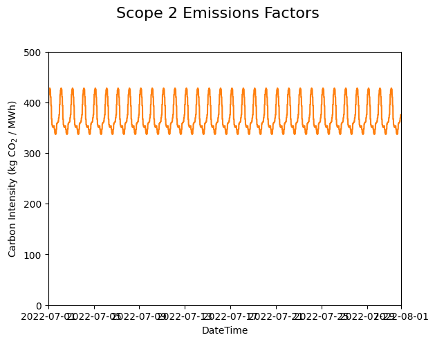
Average Scope 2 emissions factors for our modeling period (July 2022).
Next, we plot the baseline and optimal electricity consumption profiles. This helps us to visualize how the model responds to the cost incentives of the tariff.
# plot the model outputs
fig, ax = plt.subplots()
ax.step(battery.t, net_load, color="C0", lw=2, label="Net Load")
ax.step(battery.t, baseload, color="k", lw=1, ls='--', label="Baseload")
ax.set(xlabel="DateTime", ylabel="Power (kW)", xlim=(battery.start_dt, battery.end_dt))
plt.xticks(rotation=45)
fig.tight_layout()
plt.legend()
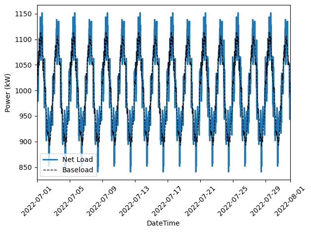
Output of our electricity bill optimization using the virtual battery model. The dotted line is baseline electricity purchases, and the blue line is the optimized profile. Note how the optimized electricity profile shaves peaks to readuce time-of-use (TOU) charges
Finally, let’s plot the battery state of charge (SOC) to confirm that the constraints were respected:
# plot the battery charge
battery_charge = np.array([battery.model.soc[t].value for t in battery.model.t])
fig, ax = plt.subplots()
ax.step(battery.t, battery_charge, color="C1", lw=2, label="Battery SOC")
ax.set(xlabel="Time", ylabel="Battery SOC", ylim=[0,1], xlim=(battery.start_dt, battery.end_dt))
plt.xticks(rotation=45)
fig.tight_layout()
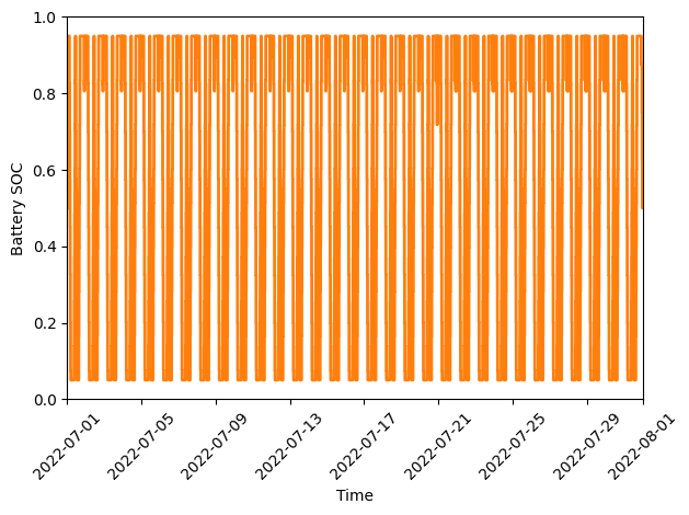
Battery state of charge (SOC) as a percentage during our modeling period (July 2022).