Optimize Electricity Costs
This tutorial will walkthrough how to optimize electricity bill savings for a simple battery model in either CVXPY or Pyomo by going through the following steps:
Load an electricity tariff spreadsheet
We publish a nationwide tariff dataset: https://github.com/we3lab/industrial-electricity-tariffs
In this case, we use tariff.csv from the EEC data folder
Configure an optimization model of the electricity consumer with system constraints
Consider using flexibility metrics to encode system constraints (Flexibility Metrics as Constraints)!
The models are presented step-by-step to demonstrate the model building process, but the complete models are available in the examples folder:
Create an objective function of electricity costs based on this tariff sheet
Minimize the electriciy costs of this consumer given the system constraints and base load consumption
Display the results to validate that the optimization is correct
CVXPY
Import dependencies
import datetime
import cvxpy as cp
import pandas as pd
import matplotlib.pyplot as plt
from electric_emission_cost import costs
Load an electricity tariff spreadsheet
path_to_tariff_sheet = "electric_emission_cost/data/tariff.csv"
tariff_df = pd.read_csv(path_to_tariff_sheet, sep=",")

# get the charge dictionary
charge_dict = costs.get_charge_dict(
    datetime.datetime(2023, 4, 9), datetime.datetime(2023, 4, 11), tariff_df, resolution="1m"
)
We are going to evaluate the electricity consumption from only April 9th to April 10th since that is where our synthetic data comes from (https://github.com/we3lab/electric-emission-cost/blob/main/electric_emission_cost/data/consumption.csv). You will also see that it is in 1-minute intervals, hence resolution=”1m”. If you print charge_dict, then you should get the following:
{
    'electric_customer_0_20230409_20230410_0': array([666.65]),
    'electric_energy_0_20230409_20230410_0': array([0., 0., 0., ..., 0., 0., 0.]),
    'electric_energy_1_20230409_20230410_0': array([0., 0., 0., ..., 0., 0., 0.]),
    'electric_energy_2_20230409_20230410_0': array([0., 0., 0., ..., 0., 0., 0.]),
    'electric_energy_3_20230409_20230410_0': array([0., 0., 0., ..., 0., 0., 0.]),
    'electric_energy_4_20230409_20230410_0': array([0. , 0. , 0. , ..., 0.0189944, 0.0189944, 0.0189944]),
    'electric_energy_5_20230409_20230410_0': array([0., 0., 0., ..., 0., 0., 0.]),
    'electric_energy_6_20230409_20230410_0': array([0., 0., 0., ..., 0., 0., 0.]),
    'electric_energy_7_20230409_20230410_0': array([0., 0., 0., ..., 0., 0., 0.]),
    'electric_energy_8_20230409_20230410_0': array([0., 0., 0., ..., 0., 0., 0.]),
    'electric_energy_9_20230409_20230410_0': array([0., 0., 0., ..., 0., 0., 0.]),
    'electric_energy_10_20230409_20230410_0': array([0., 0., 0., ..., 0., 0., 0.]),
    'electric_energy_11_20230409_20230410_0': array([0., 0., 0., ..., 0., 0., 0.]),
    'electric_energy_12_20230409_20230410_0': array([0., 0., 0., ..., 0., 0., 0.]),
    'electric_energy_13_20230409_20230410_0': array([0., 0., 0., ..., 0., 0., 0.]),
    'electric_energy_14_20230409_20230410_0': array([0.0189944, 0.0189944, 0.0189944, ..., 0. , 0. , 0. ]),
    'electric_energy_15_20230409_20230410_0': array([0., 0., 0., ..., 0., 0., 0.]),
    'electric_energy_16_20230409_20230410_0': array([0., 0., 0., ..., 0., 0., 0.]),
    'electric_demand_0_20230409_20230410_0': array([0., 0., 0., ..., 0., 0., 0.]),
    'electric_demand_1_20230409_20230410_0': array([0., 0., 0., ..., 0., 0., 0.]),
    'electric_demand_2_20230409_20230410_0': array([ 0.  ,  0.  ,  0.  , ..., 19.79, 19.79, 19.79]),
    'electric_demand_3_20230409_20230410_0': array([19.79, 19.79, 19.79, ...,  0.  ,  0.  ,  0.  ])
}
Configure an optimization model of the electricity consumer with system constraints
# load historical consumption data
load_df = pd.read_csv("electric_emission_cost/data/consumption.csv", parse_dates=["Datetime"])

# set battery parameters
# create variables for battery total energy, max charge and discharge power, and SOC limits
total_capacity = 10 # kWh
min_soc = 0
max_soc = 1
init_soc = 0.5
fin_soc = 0.5
max_discharge = 5 # kW
max_charge = 5 # kW
T = len(load_df["Datetime"])
delta_t = ((load_df.iloc[-1]["Datetime"] - load_df.iloc[0]["Datetime"]) / T) / datetime.timedelta(hours=1)

# initialize variables
battery_output_kW = cp.Variable(T)
battery_soc = cp.Variable(T+1)
grid_demand_kW = cp.Variable(T)

# set constraints
constraints = [
    battery_output_kW >= -max_discharge,
    battery_output_kW <= max_charge,
    battery_soc >= min_soc,
    battery_soc <= max_soc,
    battery_soc[0] == init_soc,
    battery_soc[T] == fin_soc,
    grid_demand_kW >= 0
]
for t in range(T):
    constraints += [
        battery_soc[t+1] == battery_soc[t] + (battery_output_kW[t] * delta_t) / total_capacity,
        grid_demand_kW[t] == load_df.iloc[t]["Load [kW]"] + battery_output_kW[t]
    ]
This is a standard battery model with energy (i.e., total charge) and power (i.e., discharge/charge rate) constraints. The round-trip efficiency is 1.0 since there is no penalty applied when discharging the battery, but that’s fine for these demonstration purposes.
Create an objective function of electricity costs based on this tariff sheet
# requires a consumption dictionary in case there is natural gas in addition to electricity
consumption_data_dict = {"electric": grid_demand_kW}
# NOTE: second entry of the tuple can be ignored since it's for Pyomo
obj, _ = costs.calculate_cost(
    charge_dict,
    {"electric": grid_demand_kW},
    resolution="1m",
    consumption_estimate=load_df["Load [kW]"].sum(),
    desired_utility="electric",
)
The charge and consumption dictionaries are relatively straightforward: charge_dict comes from the EEC package and consumption_data_dict is either an optimization variable or numpy array (in the case of historical analysis). The only caveat would be that an entry with key “gas” must be included to analzye natural gas consumption.
Carefully note that the function calculate_cost returns a tuple. The second entry of the tuple is for Pyomo, so it can be ignored since we are using CVXPY.
The resolution argument represents the temporal granularity of the data in string format. The default value is “15m” for 15-minute intervals, but our consumption data is on 1-minute intervals, so we use resolution=”1m” (just like with charge_dict).
For this simple example the prev_demand_dict, prev_consumption_dict, demand_scale_factor, desired_charge_type, and varstr_alias_func have not been used. More information on how to use those flags is available in How to Use Advanced Features.
Minimize the electriciy costs of this consumer given the system constraints and base load consumption
# solve the CVX problem (objective variable should be named obj)
prob = cp.Problem(cp.Minimize(obj), constraints)
prob.solve()
Display the results to validate that the optimization is correct
Always compute the ex-post cost using numpy due to the convex relaxations that we apply in our optimization code:
# NOTE: second entry of the tuple can be ignored since it's for Pyomo
baseline_electricity_cost, _ = costs.calculate_cost(
    charge_dict,
    {"electric": load_df["Load [kW]"].values},
    resolution="1m",
    desired_utility="electric",
)
# NOTE: second entry of the tuple can be ignored since it's for Pyomo
optimized_electricity_cost, _ = costs.calculate_cost(
    charge_dict,
    {"electric": grid_demand_kW.value},
    resolution="1m",
    desired_utility="electric",
)
Note that the consumption_estimate optional argument is not needed because the electricity consumption is a numpy array instead of an optimization variable. If we print our results, we confirm that the optimal electricity profile has a bill of $703.81, $61.48 less than the baseline bill of $765.29.
>>>print(f"Baseline Electricity Cost: ${baseline_electricity_cost:.2f}")
Baseline Electricity Cost: $765.29
>>>print(f"Optimized Electricity Cost: ${optimized_electricity_cost:.2f}")
Optimized Electricity Cost: $703.81
Below are a few simple plots to validate our results. First, we visualize the energy and demand charges:
# this can also be done in a dataframe format that drops all the unnecessary columns
charge_df = costs.get_charge_df(datetime.datetime(2023, 4, 9), datetime.datetime(2023, 4, 11), tariff_df, resolution="1m")
charge_df.head()

# create a subset of the charge_df for energy and demand charges
energy_charge_df = charge_df.filter(like="energy")
demand_charge_df = charge_df.filter(like="demand")

# sum across all energy charges
total_energy_charge = energy_charge_df.sum(axis=1)

fig, ax = plt.subplots(2, 1, figsize=(10, 8))
# plot the energy charges
ax[0].plot(charge_df["DateTime"], total_energy_charge)
ax[0].set(
    xlabel="DateTime",
    ylabel="Energy Charge ($/kWh)",
    xlim=(datetime.datetime(2023, 4, 9), datetime.datetime(2023, 4, 11))
)

# plot the demand charges
ax[1].plot(charge_df["DateTime"], demand_charge_df)
ax[1].set(
    xlabel="DateTime",
    ylabel="Demand Charge ($/kWh)",
    xlim=(datetime.datetime(2023, 4, 9),
    datetime.datetime(2023, 4, 11)),
    ylim=[0,None]
)

fig.align_ylabels()
fig.tight_layout()
fig.suptitle("Electricity Charges",y=1.02, fontsize=16)
plt.show()
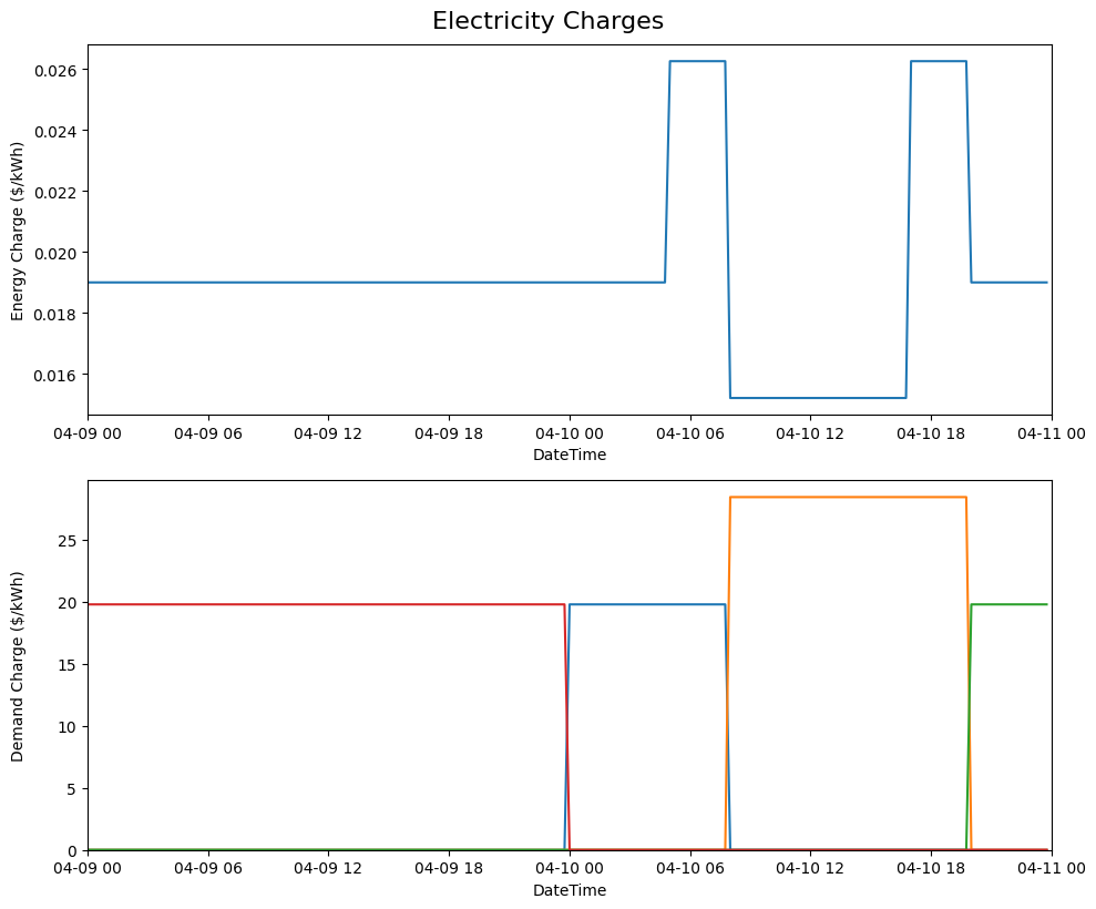
Structure of time-of-use (TOU) energy and demand charges for our modeling period (April 9-10, 2023). Different colors indicate different demand charge periods. Note that because April 9th is a Sunday, there are no TOU charges until Monday (April 10th).
Next, we plot the baseline and optimal electricity consumption profiles. This helps us to visualize how the model responds to the cost incentives of the tariff.
# plot the model outputs
fig, ax = plt.subplots()
ax.step(charge_df["DateTime"], grid_demand_kW.value, color="C0", lw=2, label="Net Load")
ax.step(charge_df["DateTime"], load_df["Load [kW]"].values, color="k", lw=1, ls='--', label="Baseload")
ax.set(xlabel="DateTime", ylabel="Power (kW)", xlim=(datetime.datetime(2023, 4, 9), datetime.datetime(2023, 4, 11)))
plt.xticks(rotation=45)
fig.tight_layout()
plt.legend()
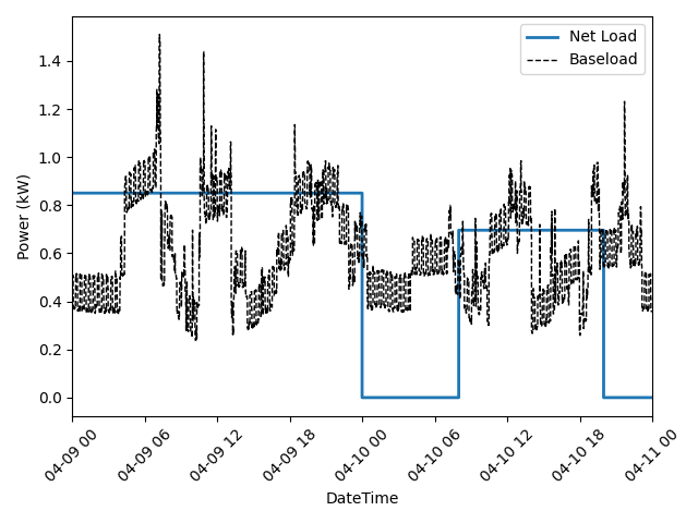
Output of our electricity bill optimization using the virtual battery model. The dotted line is baseline electricity purchases, and the blue line is the optimized profile. Note how the optimized electricity profile shaves peaks to readuce time-of-use (TOU) charges
Finally, let’s plot the battery state of charge (SOC) to confirm that the constraints were respected:
# plot the battery charge
fig, ax = plt.subplots()
ax.step(charge_df["DateTime"], battery_soc.value[1:], color="C1", lw=2, label="Battery SOC")
ax.set(
    xlabel="Time",
    ylabel="Battery SOC",
    ylim=[0,1],
    xlim=(datetime.datetime(2023, 4, 9), datetime.datetime(2023, 4, 11))
)
plt.xticks(rotation=45)
fig.tight_layout()
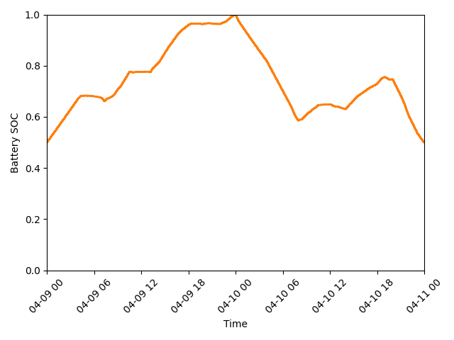
Battery state of charge (SOC) as a percentage during our modeling period (April 9-10, 2023).
Pyomo
Import dependencies
import datetime
import numpy as np
import pandas as pd
import matplotlib.pyplot as plt
from electric_emission_cost import costs
from examples.pyomo_battery_model import BatteryPyomo
Load an electricity tariff spreadsheet
path_to_tariffsheet = "electric_emission_cost/data/tariff.csv"
tariff_df = pd.read_csv(path_to_tariffsheet, sep=",")

# get the charge dictionary
charge_dict = costs.get_charge_dict(
    datetime.datetime(2022, 7, 1), datetime.datetime(2022, 8, 1), tariff_df, resolution="15m"
)
We are going to evaluate the electricity consumption for the entire month of July 2022. Below we will create synthetic baseload data for this month with 15-minute resolution, so resolution=”15m”. If you print charge_dict, then you should get the following:
{
    'electric_customer_0_2022-07-01_2022-07-31_0': array([666.65]),
    'electric_energy_0_2022-07-01_2022-07-31_0': array([0., 0., 0., ..., 0., 0., 0.], shape=(2976,)),
    'electric_energy_1_2022-07-01_2022-07-31_0': array([0., 0., 0., ..., 0., 0., 0.], shape=(2976,)),
    'electric_energy_2_2022-07-01_2022-07-31_0': array([0., 0., 0., ..., 0., 0., 0.], shape=(2976,)),
    'electric_energy_3_2022-07-01_2022-07-31_0': array([0., 0., 0., ..., 0., 0., 0.], shape=(2976,)),
    'electric_energy_4_2022-07-01_2022-07-31_0': array([0., 0., 0., ..., 0., 0., 0.], shape=(2976,)),
    'electric_energy_5_2022-07-01_2022-07-31_0': array([0.0254538, 0.0254538, 0.0254538, ..., 0. , 0. , 0. ], shape=(2976,)),
    'electric_energy_6_2022-07-01_2022-07-31_0': array([0., 0., 0., ..., 0., 0., 0.], shape=(2976,)),
    'electric_energy_7_2022-07-01_2022-07-31_0': array([0., 0., 0., ..., 0., 0., 0.], shape=(2976,)),
    'electric_energy_8_2022-07-01_2022-07-31_0': array([0., 0., 0., ..., 0., 0., 0.], shape=(2976,)),
    'electric_energy_9_2022-07-01_2022-07-31_0': array([0., 0., 0., ..., 0., 0., 0.], shape=(2976,)),
    'electric_energy_10_2022-07-01_2022-07-31_0': array([0., 0., 0., ..., 0., 0., 0.], shape=(2976,)),
    'electric_energy_11_2022-07-01_2022-07-31_0': array([0., 0., 0., ..., 0., 0., 0.], shape=(2976,)),
    'electric_energy_12_2022-07-01_2022-07-31_0': array([0., 0., 0., ..., 0., 0., 0.], shape=(2976,)),
    'electric_energy_13_2022-07-01_2022-07-31_0': array([0., 0., 0., ..., 0., 0., 0.], shape=(2976,)),
    'electric_energy_14_2022-07-01_2022-07-31_0': array([0., 0., 0., ..., 0., 0., 0.], shape=(2976,)),
    'electric_energy_15_2022-07-01_2022-07-31_0': array([0. , 0. , 0. , ..., 0.0254538, 0.0254538, 0.0254538], shape=(2976,)),
    'electric_energy_16_2022-07-01_2022-07-31_0': array([0., 0., 0., ..., 0., 0., 0.], shape=(2976,)),
    'electric_demand_0_2022-07-01_2022-07-31_0': array([19.79, 19.79, 19.79, ...,  0.  ,  0.  ,  0.  ], shape=(2976,)),
    'electric_demand_1_2022-07-01_2022-07-31_0': array([0., 0., 0., ..., 0., 0., 0.], shape=(2976,)),
    'electric_demand_2_2022-07-01_2022-07-31_0': array([0., 0., 0., ..., 0., 0., 0.], shape=(2976,)),
    'electric_demand_3_2022-07-01_2022-07-31_0': array([ 0.  ,  0.  ,  0.  , ..., 19.79, 19.79, 19.79], shape=(2976,))
}
Configure an optimization model of the electricity consumer with system constraints
We rely on the virtual battery model in pyomo_battery_model.py. We’re going to stick to the electricity cost calculation details, but we encourage you to go check out the code to better understand the model.
# Define the parameters for the battery model
battery_params = {
    "start_date": "2022-07-01 00:00:00",
    "end_date": "2022-08-01 00:00:00",
    "timestep": 0.25,   # 15 minutes defined in hours
    "rte": 0.86,
    "energycapacity": 100,
    "powercapacity": 50,
    "soc_min": 0.05,
    "soc_max": 0.95,
    "soc_init": 0.5,
}

# Create a sample baseload profile based on a sine wave
baseload = np.sin(np.linspace(0, 4 * np.pi, 96))*100 + 1000 + np.random.normal(0, 10, 96)

# Create an instance of the BatteryOpt class
battery = BatteryPyomo(battery_params, baseload, baseload_repeat=True)

# create the model on the instance battery
battery.create_model()
The above code initializes the battery model with flexibility metrics like round-trip efficiency (RTE), power capacity, and energy capacity.
Create an objective function of electricity costs based on this tariff sheet
# monthly total consumption - divided by 4 because of 15-min resolution
consumption_estimate = sum(baseload) / 4
# this example tariff only has electric utility types so we do not pass the gas key
consumption_data_dict = {"electric": battery.model.net_facility_load}
battery.model.electricity_cost, battery.model = costs.calculate_cost(
    charge_dict,
    consumption_data_dict,
    resolution="15m",
    consumption_estimate=consumption_estimate,
    desired_utility="electric",
    model=battery.model,
)
# create an attribute objective based on the electricity cost
battery.model.objective = pyo.Objective(
    expr=battery.model.electricity_cost,
    sense=pyo.minimize,
)
Minimize the electriciy costs of this consumer given the system constraints and base load consumption
# use the glpk solver to solve the model - (any pyomo-supported LP solver will work here)
solver = pyo.SolverFactory("glpk")
results = solver.solve(battery.model, tee=False) # turn tee=True to see solver output
Display the results to validate that the optimization is correct
Always compute the ex-post cost using numpy due to the convex relaxations that we apply in our optimization code:
# retrieve outputs from Pyomo model
net_load = np.array([battery.model.net_facility_load[t].value for t in battery.model.t])
baseload = np.array([battery.model.baseload[t] for t in battery.model.t])
# NOTE: second entry of the tuple can be ignored since it's for Pyomo
baseline_electricity_cost = costs.calculate_cost(
    charge_dict,
    {"electric": baseload},
    resolution="15m",
    desired_utility="electric",
)
# NOTE: second entry of the tuple can be ignored since it's for Pyomo
optimized_electricity_cost, _ = costs.calculate_cost(
    charge_dict,
    {"electric": net_load},
    resolution="15m",
    desired_utility="electric",
)
Note that the consumption_estimate optional argument is not needed because the electricity consumption is a numpy array instead of an optimization variable. If we print our results, we confirm that the optimal electricity profile has a bill of $113384.23, $2182.47 less than the baseline bill of $115566.70.
>>>print(f"Baseline Electricity Cost: ${baseline_electricity_cost:.2f}")
Baseline Electricity Cost: $115566.70
>>>print(f"Optimized Electricity Cost: ${optimized_electricity_cost:.2f}")
Optimized Electricity Cost: $113384.23
Below are a few simple plots to validate our results. First, we visualize the energy and demand charges:
# this can also be done in a dataframe format that drops all the unnecessary columns
charge_df = costs.get_charge_df(battery.start_dt, battery.end_dt, tariff_df, resolution="15m")
charge_df.head()

# create a subset of the charge_df for energy and demand charges
energy_charge_df = charge_df.filter(like="energy")
demand_charge_df = charge_df.filter(like="demand")

# sum across all energy charges
total_energy_charge = energy_charge_df.sum(axis=1)

fig, ax = plt.subplots(2, 1, figsize=(10, 8))
# plot the energy charges
ax[0].plot(charge_df["DateTime"], total_energy_charge)
ax[0].set(xlabel="DateTime", ylabel="Energy Charge ($/kWh)", xlim=(battery.start_dt, battery.end_dt))

# plot the demand charges
ax[1].plot(charge_df["DateTime"], demand_charge_df)
ax[1].set(xlabel="DateTime", ylabel="Demand Charge ($/kWh)", xlim=(battery.start_dt, battery.end_dt), ylim=[0,None])

fig.align_ylabels()
fig.tight_layout()
fig.suptitle("Electricity Charges",y=1.02, fontsize=16)
plt.show()
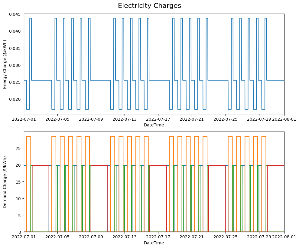
Structure of time-of-use (TOU) energy and demand charges for our modeling period (July 2022).
Next, we plot the baseline and optimal electricity consumption profiles. This helps us to visualize how the model responds to the cost incentives of the tariff.
# plot the model outputs
fig, ax = plt.subplots()
ax.step(charge_df["DateTime"], net_load, color="C0", lw=2, label="Net Load")
ax.step(charge_df["DateTime"], baseload, color="k", lw=1, ls='--', label="Baseload")
ax.set(xlabel="DateTime", ylabel="Power (kW)", xlim=(battery.start_dt, battery.end_dt))
plt.xticks(rotation=45)
fig.tight_layout()
plt.legend()
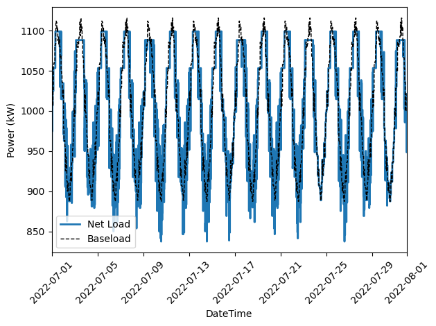
Output of our electricity bill optimization using the virtual battery model. The dotted line is baseline electricity purchases, and the blue line is the optimized profile. Note how the optimized electricity profile shaves peaks to readuce time-of-use (TOU) charges
Finally, let’s plot the battery state of charge (SOC) to confirm that the constraints were respected:
# plot the battery charge
battery_charge = np.array([battery.model.soc[t].value for t in battery.model.t])
fig, ax = plt.subplots()
ax.step(charge_df["DateTime"], battery_charge, color="C1", lw=2, label="Battery SOC")
ax.set(xlabel="Time", ylabel="Battery SOC", ylim=[0,1], xlim=(battery.start_dt, battery.end_dt))
plt.xticks(rotation=45)
fig.tight_layout()
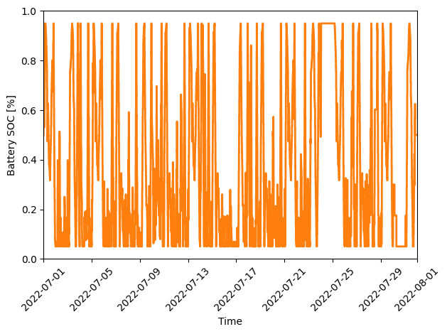
Battery state of charge (SOC) as a percentage during our modeling period (July 2022).